In this guide
- Design the monitoring around a decision
- Chemistry: What to Sample, Where, and When
- Internal vs External: The Mass-Balance Answer
- Real-time buoys and sensor placement
- Satellite monitoring and lake history
- Predictive models and early warning
- Post-Treatment: What to Measure and When
- Laboratory analysis, in-house capability, and technical evidence
- References & resources
01Design the monitoring around a decision
The most useful monitoring program changes what happens next. An oxygen record may show that an existing system needs a different operating window, while a phosphorus budget may reveal that a proposed sediment treatment would miss the larger inflow source. Compliance and long-term trend records still have their own value, but we design diagnostic monitoring around the decision it needs to resolve.
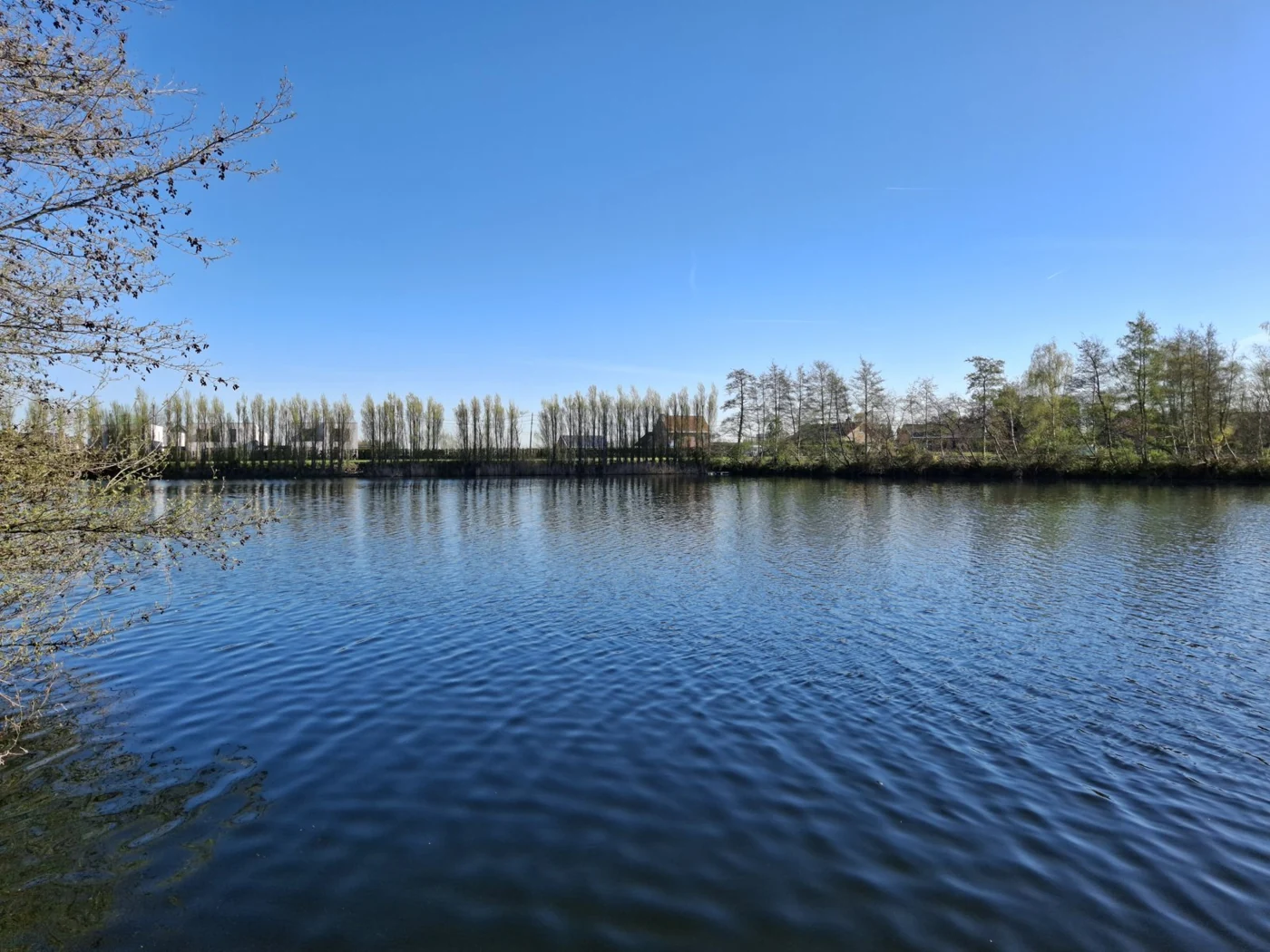
Ruling out an explanation can be as valuable as confirming one. If bottom water stays oxygenated through two summers, extensive water-column anoxia becomes a less convincing explanation for the bloom. That directs attention to inflows, high-pH release, decomposition, and reducing sediment below the oxygenated water, rather than supporting an automatic purchase of more aeration. The value is the better next decision, not simply another completed sampling season.
A lake's history often contains the first useful clues: profiles, laboratory results, treatment dates, rainfall, lake levels, and observations of where a bloom appeared. We can work from those records as they are; matching dates, depths, and methods is part of our review.
The output should connect an observation to a practical decision, with sufficient lead time and a responsible person. An alert about low oxygen is most useful when it leads to a defined response, such as confirming conditions, adjusting an existing operation, or investigating a constituent risk. The threshold and response need to fit the site.
| Question | Evidence with a distinct role | Decision it can support |
|---|---|---|
| What sustains recurring blooms? | Seasonal nutrient sources, sediment behavior, biological composition and transport | Whether to prioritize watershed, sediment or biological management |
| What is approaching the intake? | Depth profiles, constituent samples, withdrawal conditions and inflow events | Intake operation and preparation at the plant |
| Is the treatment working? | A baseline, treatment records, comparison observations and the intended endpoint | Continue, modify, expand or stop an intervention |
| Can an event be anticipated? | Consistent historical records, continuous data and independently tested prediction | A response with useful lead time and known uncertainty |
The same instrument can contribute to several questions, but collecting more readings doesn't automatically distinguish their causes. [1] [2]
We develop a conceptual explanation of the lake before selecting the instruments. It describes plausible sources, the conditions that change them, and the routes by which they affect the place of concern. Monitoring then distinguishes between competing explanations. A sample that doesn't discriminate between them may still be useful for compliance, but it has a different role.
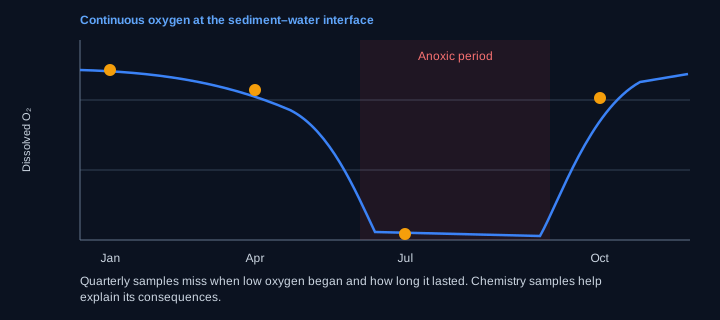
Quarterly visits can miss the onset and duration of a short anoxic period even if one sample catches low oxygen. Continuous measurements explain what happened between visits; targeted laboratory samples explain the chemical consequences. Pairing the two can be more informative than increasing the number of analytes in the same infrequent visit. [3]
Schedule a call about the question your monitoring needs to answer →
02Chemistry: What to Sample, Where, and When
A lake isn't one uniform sample. Temperature stratification can separate warm surface water from deeper water for extended periods. Oxygen, phosphorus, manganese, and odor compounds can vary sharply across that boundary. Wind, inflows, water-level changes, and withdrawal can alter those distributions.
A surface sample can describe a swimming area while missing a deep chlorophyll maximum or the water approaching an intake. We use profiles to locate those layers, then collect discrete samples where they answer the question. An inlet visit during storm flow can be more useful for source assessment than another dry-weather sample, while time-of-day oxygen and pH measurements help interpret shallow-water biological activity.
Timing matters on several scales. Seasonal observations describe stratification and recovery; event sampling can capture inflow pulses; continuous sensors reveal short oxygen or pH changes. High daytime pH and oxygen may reflect photosynthesis, but they don't identify the organism responsible. A low pre-dawn oxygen measurement can establish a habitat concern without proving whether plants, algae, or sediment demand is the main cause.
Chemical form can change the interpretation of the same reported concentration. Whole-water and filtered samples separate particulate material from an operationally defined dissolved fraction; that distinction is useful for phosphorus, manganese, and odor compounds. Filtration, preservation, and handling need to be agreed with the laboratory because delayed processing or damaged cells can change the fraction being measured.
Sediment fractionation and intact-core work complement water samples. Fractionation separates the phosphorus into labile, iron-bound, organic, aluminum-bound, calcium-or-lanthanum, and residual fractions; incubations measure release under selected conditions. The iron-bound and organic fractions carry most of the release potential, so total sediment phosphorus is a poor substitute for either measurement (see Sediment Phosphorus and Internal Loading). Neither replaces field context. Oxygenated bottom water doesn't rule out phosphorus release from high pH, decomposition, disturbance, or reducing microsites below the interface.
| Measurement | What the distinction reveals | Interpretation issue |
|---|---|---|
| Total P, total dissolved P and soluble reactive P | Particle-associated, dissolved and readily reactive fractions | Methods define the fractions; soluble reactive P is not all potentially bioavailable P. |
| Total N, ammonium, nitrate and nitrite | Nutrient supply and transformations under different oxygen conditions | A ratio using totals is not equivalent to a ratio using dissolved inorganic nutrients. |
| Dissolved and total manganese or iron | Soluble constituents versus particles requiring different removal barriers | Filtration, preservation and oxidation during handling can alter the apparent distribution. |
| Temperature and dissolved oxygen profiles | Stratification, habitat and the setting for chemical transformations | Sensor depth and bottom clearance must be interpretable against changing water level. |
| pH, alkalinity and conductivity | Acid-base conditions, buffering and changes in dissolved constituents | pH is not buffering capacity; conductivity does not identify the individual ions. |
| Chlorophyll-a, phycocyanin and microscopy | Biomass-related signals and community identity | Pigment content varies; microscopy identifies organisms but does not quantify toxin concentration. |
| TOC/DOC, UV absorbance, geosmin/MIB and toxins | Organic matter and specific source-water constituents | Bulk carbon and odor are not substitutes for compound-specific analysis. |
Analyte selection, methods, sampling coverage and quality controls are chosen to resolve the management question. [3] [2] [15]
Reporting limits deserve attention before a sample is collected. “Not detected” means below the method's reporting capability, not absent. A reporting limit above the concentration relevant to the management decision can't establish that the condition is acceptable. Field duplicates, blanks and laboratory quality controls help separate an environmental change from analytical or sampling variability.
ENV selects the combination of profiles, water analyses, sediment work, and biological observations needed to resolve the question. Detection limits, sample preservation, contamination controls, and method consistency are part of that design.
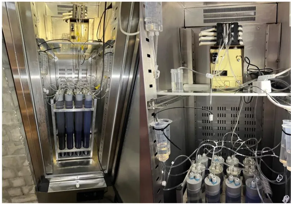
Field observations also help select sediment samples. Color, texture, organic material, and reported sulfide odors can distinguish areas that deserve separate analysis, particularly when a sheltered cove differs from an exposed shore. Those observations guide representative sampling and the chemistry needed to interpret it. An experienced sediment specialist can use them to estimate release risk qualitatively before laboratory analysis is purchased, but only if the sediment is described immediately upon collection, because color and texture change once it is exposed to air. Refrigerated samples then keep their phosphorus forms for laboratory analysis with minimal change.
Discuss your sampling locations, depths, and available results →
03Internal vs External: The Mass-Balance Answer
A high phosphorus concentration at one station and a large phosphorus load to the lake aren't the same result. We connect concentrations with water volume or flow, and put the measurements on the same seasonal timeline. That allows a comparison between a tributary supplying the lake during storms and sediment supplying it through the dry growing season.
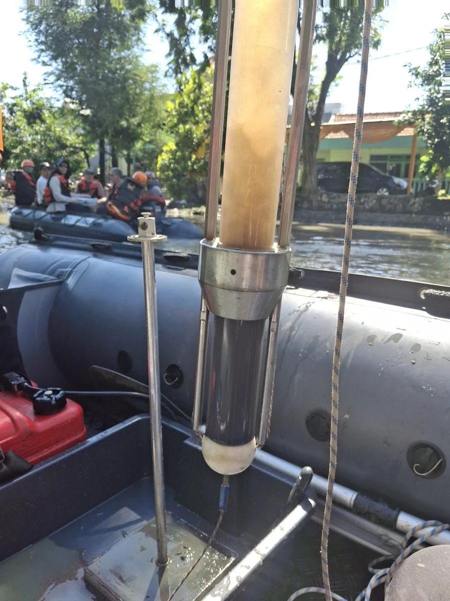
External sources can include stormwater, tributaries, groundwater, direct deposition, and wastewater inputs. Their relative importance may change with season. High-flow events can deliver substantial particulate material, while a less conspicuous continuous inflow may contribute dissolved nutrients throughout the growing period.
Early- and late-stratification profiles can show how much phosphorus has accumulated in the deep-water volume. Paired with oxygen, inflow, and withdrawal records, that accumulation is a useful starting estimate for the source assessment. The budget then accounts for settling, exchange across the thermocline, and changing layer volume so that accumulation isn't simply relabeled as sediment release.
Shallow lakes can recycle phosphorus without a persistent accumulation at depth. Wind resuspension, benthic organisms, high pH, and rapid biological uptake can obscure the source in routine water samples. Spatial sediment data and observations during relevant events can therefore be more informative than adding more surface samples on the same schedule.
A nutrient budget combines these lines of evidence and identifies uncertain terms. It may not close exactly. The useful outcome is an estimate that distinguishes major sources well enough to guide investment and shows which remaining uncertainty could change the recommendation.
Mass balance connects concentration with sources
A phosphorus budget accounts for changes in the mass stored in the water, together with inputs and outputs over the same period. In conceptual form:
Change in water-column P storage = external inputs + upward sediment transfer − outflow export − settling to sediment.
Upward sediment transfer includes dissolved release and resuspension. It's shown separately from settling, so deposition is counted once. The budget estimates these exchanges over the same period and within a clearly defined boundary.
The terms depend on the boundary being assessed. A whole-lake budget and a hypolimnetic budget have different transport terms. In the latter, exchange across the thermocline matters. Biological uptake redistributes phosphorus among dissolved and particulate forms; it doesn't remove total phosphorus from the water column unless material settles, is harvested or otherwise crosses the chosen boundary. [4]
| Budget component | Evidence | Common source of uncertainty |
|---|---|---|
| External inputs | Flow and phosphorus concentration in relevant inflows, runoff and other sources | Missed storms, groundwater, short concentration peaks and ungauged inputs |
| Change in storage | Concentration by depth and the corresponding water volumes | Changing lake level, stratification and inconsistent depth coverage |
| Export | Outflow or withdrawal volume and its phosphorus concentration | Using a surface concentration for a deeper withdrawal |
| Sediment exchange | Core experiments, sediment chemistry and field accumulation | Spatial variation and differences between gross release and net retention |
| Settling and vertical exchange | Evidence of particles, mixing and movement between layers | Treating every increase at depth as new sediment release |
An unexplained budget residual can indicate internal loading, but it also includes errors and omitted terms. Independent sediment evidence helps test the interpretation. [4]
Source importance can change during the year. An annual budget dominated by runoff can still contain a summer period when sediment supplies much of the immediately available phosphorus. We use the budget period that matches the management problem, while retaining the annual view needed to understand replenishment and durability. [5]
We use the budget to compare the portion of loading that each intervention can influence. That prevents a treatment from being assessed against all phosphorus entering the lake when it only targets one source or one season.
Talk through what your seasonal profiles reveal about sources →
04Real-time buoys and sensor placement
A continuous station dates the onset, duration, and recovery of an event that may occur entirely between sampling visits. A cool spell can mix nutrient-rich bottom water upward and the lake can restratify before the next monthly visit. Oxygen and temperature at the affected depths make that event visible while there's still time to collect a useful sample or change an operation.
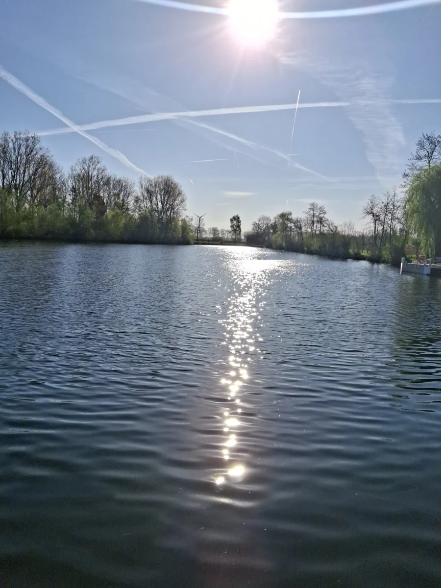
Placement determines what the system can detect. A surface instrument describes surface conditions. A deep instrument may detect an oxygen problem but miss a bloom near shore. A fixed-depth sensor can move from one thermal layer to another as the thermocline or lake level changes. Multiple depths or a profiling system may be appropriate where vertical movement matters.
For a stratified basin, we usually want a measurement close enough to the sediment-water interface to detect developing oxygen loss, while keeping the probe clear of sediment and local diffuser effects. A mid-depth oxygen minimum needs its own sensor. The actual depths follow the profile and intake configuration: a fixed two-meter offset from the bed doesn't reliably select the relevant layer in every lake.
Fouling and calibration drift need different corrections. Cleaning can reveal the effect of material growing on a probe; a subsequent standard or independent check reveals whether the sensor's calibration has also shifted. Keeping those observations separate helps us distinguish a real oxygen event from an instrument trend, rather than smoothing away the signal the buoy was installed to capture. [3]
Continuous records reveal events that routine visits miss
Fluorescence provides rapid pigment-related measurements, not a direct species count. Light history, temperature, suspended matter and the pigment content of the community can affect the signal. Laboratory chlorophyll, microscopy or toxin analysis can provide independent checks where the decision requires them. A buoy is especially useful when these records are interpreted together. [2]
Top- and bottom-water DO and temperature monitoring can be configured for under $5,000 in the entry-level setups described in ENV's project experience. Installation, servicing, telemetry, and additional sensors depend on the site and need their own scope. We start with the event the system must detect, then choose a configuration and maintenance plan that can keep detecting it through the season.
05Satellite monitoring and lake history
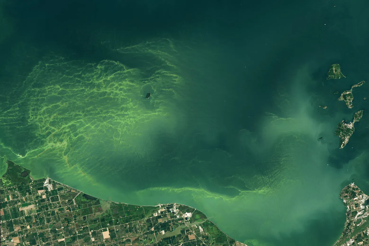
A buoy tells us what happened at its station; satellite imagery shows where the surface expression appeared across the lake. Repeated blooms in a sheltered arm, a plume following an inflow, or accumulation along a windward shore lead to different field questions. The historical archive can also put a recent treatment season beside years of earlier behavior.
The Landsat archive extends back decades. Landsat 8 has a nominal 16-day repeat cycle, with Landsat 9 offset to improve combined opportunities. Sentinel-2 provides finer spatial detail in relevant bands and a nominal five-day revisit for the constellation. Clouds, haze, sun glint, and unsuitable viewing conditions reduce usable observations.
Image availability isn't the same as a validated water-quality record. Atmospheric correction, shoreline contamination, mixed pixels, water color, suspended sediment, and differences between sensors can affect the interpretation. A small lake or narrow cove may not provide enough uncontaminated water pixels for a reliable estimate.
Chlorophyll-related indices and color changes can indicate bloom conditions, but performance needs local evaluation. Sentinel-2 doesn't have the dedicated band near 620 nm used by some sensors to help distinguish phycocyanin. An empirical relationship with cyanobacteria can be useful without being a direct measurement of that pigment. Coarser sensors may offer relevant spectral information but be unsuitable for small water bodies.
Satellite reflectance doesn't directly establish toxin concentration, species identity, bottom-water oxygen, or phosphorus release. A surface accumulation can be important for exposure while revealing little about the deeper water. Pairing imagery with field observations is what makes the historical interpretation defensible.
Our satellite work can reconstruct bloom timing and spatial patterns, identify candidate hotspots, or support a monitoring and alert program. We report the usable coverage and uncertainty alongside the pattern, so an apparent gap or trend isn't mistaken for a condition the imagery could not observe.
| Mission or sensor | Spatial and temporal context | What it contributes |
|---|---|---|
| Landsat 8 and 9 | 30 m multispectral imagery; each satellite repeats in 16 days, with an 8-day offset between them. | A long archive and lake-wide spatial comparisons; usable images depend on cloud and acquisition conditions. |
| Sentinel-2 MSI | 10, 20 and 60 m bands; nominal five-day revisit with the two-satellite constellation. | Finer spatial detail, including red-edge information useful for some water-quality applications. |
| Sentinel-3 OLCI | Approximately 300 m full-resolution pixels and an ocean-color band near 620 nm. | Spectral information relevant to phycocyanin in sufficiently large water bodies; shoreline mixing limits small-lake use. |
Pixel size isn't the size of the smallest reliable bloom measurement. Band selection, atmospheric correction, clouds, adjacency and validation determine what is interpretable. [6] [7] [8] [9]
Spatial resolution places a real limit on national products. A 2022 U.S. analysis identified 2,192 lakes resolvable with 300 m MERIS/OLCI imagery under its screening criteria. Many smaller lakes and narrow coves need a finer-resolution approach, and shore contamination still matters. The appropriate sensor follows the waterbody and question, rather than the availability of a national map. [14]
.jpg)
06Predictive models and early warning
A forecast is worth developing when its warning arrives early enough for someone to act. We work backward from that response: adjusting oxygenation, changing a withdrawal depth, arranging confirmation sampling, or preparing for a likely bloom. Predicting a condition after the useful response window has closed adds little operational value, even if the historical fit looks impressive.
A model can represent heat exchange, mixing, and nutrient cycling directly, or learn relationships between observed weather, chemistry, and biological response. We choose between those approaches according to the question and the record available. A more elaborate model is useful when it captures a process that changes the decision, not simply because it produces a more detailed dashboard.
Weather, temperature profiles, water level, inflows, operating records, and chemistry can all contribute. Their predictive value depends on the site. A relationship observed during one season may fail during an unusual storm, a treatment change, or a shift in the biological community.
About a year of overlapping real-time and satellite observations can make an initial model feasible when it captures the relevant events; many programs need several years to represent their seasonal and weather variability. That's a planning expectation from ENV's experience, not a substitute for validation. We test the model on observations it wasn't fitted to and examine missed events, false alarms, and warning time before relying on it operationally.
Early-warning performance includes lead time, missed events, false alarms, and the consequences of each. A model can fit historical measurements closely while providing little operational warning. A simpler indicator may be more useful when it's reliable and tied to a feasible response.
| Performance question | Evidence to examine |
|---|---|
| How early is the warning? | Lead time before the event, after allowing for data delay and the time needed to act |
| How often are events missed? | Sensitivity to the relevant events, including unusual seasons |
| How often is an alert unnecessary? | False alerts and their operational cost |
| Does it work on new data? | Validation on withheld time periods or events, not only the data used to fit the model |
| What changes invalidate it? | New equipment, altered withdrawal, treatment changes or a community shift |
An oxygen forecast and a toxin forecast require different observations and validation. [1] [3]
ENV develops forecasts with explicit limits and a process for updating them as new evidence arrives. An alert should state what is suspected, how uncertain it is, and whether confirmation or an operational response is appropriate. Forecasts support professional decisions; they don't replace toxin testing or establish that water is safe.
Discuss your existing record and the warning time you need →
07Post-Treatment: What to Measure and When
Treatment evaluation follows the mechanism through to the outcome. For an oxygen system, that means checking where oxygen reaches, what happens to manganese or phosphorus, and whether the resulting water quality meets the project objective. A running compressor and a high oxygen reading beside a diffuser are useful operating observations, but the investment was made for a wider benefit.
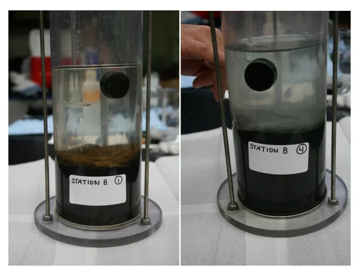
For oxygenation, the first observations include delivered oxygen and its distribution. The next include sediment conditions and constituent responses. Improved habitat, lower manganese at an intake, and reduced algae may require different locations and timescales to evaluate.
For a phosphorus treatment, immediate clearing can show flocculation or removal from the water column. Evidence of reduced internal loading requires a longer view of release and relevant water quality. Continuing inflow loads, untreated areas, seasonal mixing, and biological changes can influence the outcome.
A constituent response also needs chemical interpretation. Manganese can persist after oxygen improves because oxidation and removal aren't instantaneous under all conditions. That delay isn't proof that oxygenation failed, but it's also not a reason to disregard persistent manganese at the intake. Concentration, transport, chemistry, and the intended operating target need to be assessed together.[10]
| Intervention | Early response | Response that needs longer evaluation |
|---|---|---|
| Phosphorus binder | Distribution, water chemistry and the targeted phosphorus forms | Sediment release during relevant conditions, new inputs and biological response |
| Oxygenation | Oxygen distribution, temperature and system operation | Constituent response, habitat availability and seasonal energy or oxygen use |
| Algaecide or vegetation treatment | Target-organism response, oxygen and relevant toxin considerations | Regrowth, biomass decomposition, nutrient recycling and desirable vegetation |
| Watershed measure | Changes in delivered load during relevant flow conditions | Lake response through seasons and continuing sediment recycling |
| Source-water management | Intake quality and the immediate process response | Chemical use, filter performance, event frequency and reliability under comparable production |
“When” follows the expected process: immediate application effects, the subsequent biological or chemical response, and performance through the season that originally caused the problem. Fixed sampling intervals require site-specific design. [11] [12] [13]
A before-and-after comparison is stronger when it includes weather, inflow, lake level, treatment operation and an appropriate untreated or historical comparison. Comparing unlike seasons can make a weak treatment look effective or obscure a useful one. We select the evaluation endpoint before treatment so the program can answer the original performance question.
We use performance evaluation to identify whether to continue, adjust, expand, or discontinue an intervention. The analysis should make the reasons visible, including cases where the available evidence doesn't yet separate competing explanations.
The longest comparable record often gives the strongest baseline. Three years of monthly Secchi depth may be more useful for evaluating a clarity improvement than a new chlorophyll series started just before treatment. We can work from the records already available, match seasons and locations, and identify the additional measurements needed to explain the response. [1]
08Laboratory analysis, in-house capability, and technical evidence
The laboratory program starts with what the result needs to distinguish. A precise total measurement won't resolve a question about a dissolved fraction, while a simple, consistent field measurement may be enough to track a useful change. We separate compliance requirements, diagnostic analyses, and routine screening so each has a clear purpose and quality standard.
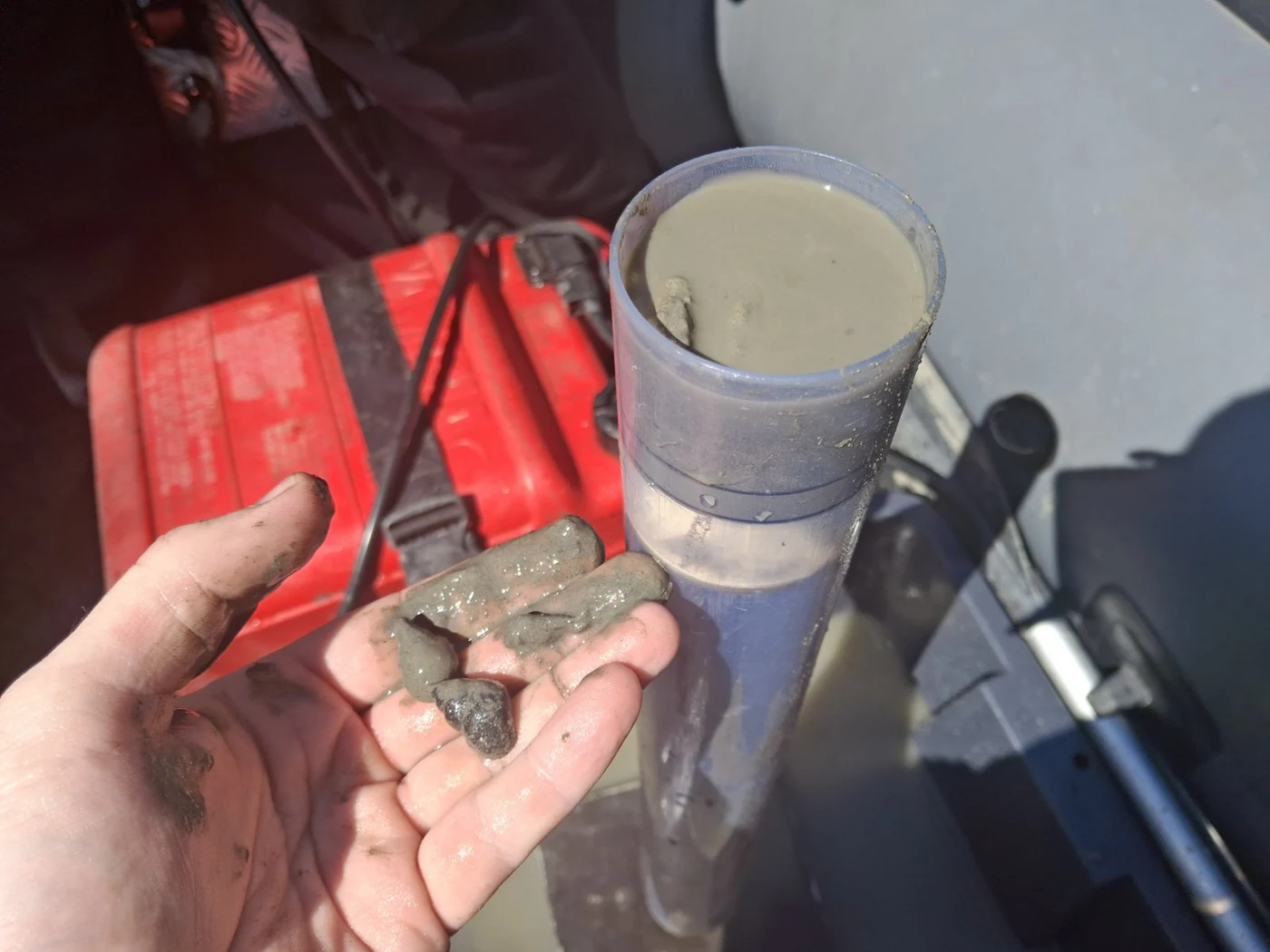
The choice between in-house and contract analysis includes equipment, staff time, training, standards, quality control, maintenance, sample volume, and reporting requirements. Specialized or accredited analyses may remain external even where routine screening is brought in-house. Screening and compliance results shouldn't be treated as interchangeable.
Building in-house capability
ENV can help select methods, develop standard procedures, train staff, and connect laboratory data with profiles, weather, and plant or lake operations. The goal is reliable interpretation as well as sample throughput. Training includes recognition of questionable results and a clear route for confirmation.
Documented methods, blanks, standards, duplicates, instrument checks, and sample traceability make results easier to compare over time. Staff turnover and method changes need to be reflected in that record. A dashboard is useful when the underlying measurements and units remain traceable.
Independent technical evidence and expert review
Water-quality disputes can involve source attribution, treatment performance, sediment chemistry, algal events, or effects on drinking-water supply. A defensible review distinguishes what was measured, what was inferred, and what remains uncertain. Sampling representativeness, chain of custody, method suitability, chronology, and alternative explanations can be as important as a single reported concentration.
For an in-house laboratory, a dependable result includes a documented method, suitable calibration, reporting units, detection capability, reference checks and a clear record of sample handling. Training can make routine measurements more useful while defining which analyses should remain with a specialist laboratory. Independent verification is particularly valuable when a method is first introduced or when results approach an action threshold. [3] [2]
ENV provides independent technical review, expert-witness services, and litigation support in these areas. We evaluate the evidence and its limits without assuming the conclusion. Engagements for either party are subject to conflict screening. The same standard of traceable reasoning is useful for a capital-investment review or a treatment-performance assessment outside litigation.
For many teams, a useful in-house starting point is Secchi depth, a maintained sonde, appropriate field colorimetry, and careful observations of sediment and bloom behavior. Specialist analyses then address the questions those observations raise. We sell no chemicals and no equipment; the recommendation is the product. Training and method selection should make existing staff more effective, rather than create a laboratory they don't need.
References & resources
Research and technical guidance supporting this guide. Advisory and regulatory information checked September 2026; local requirements may differ.
- Williams, Szaro & Shapiro (2009 printing). Adaptive Management: The U.S. Department of the Interior Technical Guide. ↩
- Chorus & Welker, editors (2021). Toxic Cyanobacteria in Water, 2nd edition. ↩
- Wagner, Boulger, Oblinger & Smith (2006). Guidelines and standard procedures for continuous water-quality monitors: Station operation, record computation, and data reporting. ↩
- Nürnberg (2009). Assessing internal phosphorus load: Problems to be solved. ↩
- Søndergaard, Jensen & Jeppesen (2003). Role of sediment and internal loading of phosphorus in shallow lakes. ↩
- U.S. Geological Survey (mission documentation). Landsat 8. ↩
- U.S. Geological Survey (mission documentation). What are the acquisition schedules for the Landsat satellites?. ↩
- European Space Agency (mission documentation). Sentinel-2: Facts and figures. ↩
- Copernicus Data Space Ecosystem (instrument documentation). Sentinel-3 OLCI L1B. ↩
- Bryant, Hsu-Kim, Gantzer & Little (2011). Solving the problem at the source: Controlling Mn release at the sediment-water interface via hypolimnetic oxygenation. ↩
- Huser et al. (2016). Longevity and effectiveness of aluminum addition to reduce sediment phosphorus release and restore lake water quality. ↩
- Singleton & Little (2006). Designing hypolimnetic aeration and oxygenation systems: A review. ↩
- U.S. EPA (2015). Recommendations for Public Water Systems to Manage Cyanotoxins in Drinking Water. ↩
- Schaeffer et al. (2022). Satellites quantify the spatial extent of cyanobacterial blooms across the United States at multiple scales. ↩
- U.S. Geological Survey (National Field Manual). National Field Manual for the Collection of Water-Quality Data. ↩
Let's talk about your monitoring data
We can review your monitoring program, investigate a specific uncertainty, or connect field measurements, satellites, and laboratory results with practical decisions.
A conversation can start with what you've observed. Existing sampling results, sensor records, or a specific question are useful starting points for deciding what the monitoring needs to resolve.
Schedule a conversation